OpenCV: optical character recognition
We will use OpenCV (http://www.opencv.org/) for optical character
recognition (OCR) using support vector machine (SVM) classifiers. This
example is based on OpenCV’s digit tutorial (available in
OPENCV_ROOT/samples/python2/digits.py).
We start with the necessary imports.
import cv2
import numpy as np
import optunity
import optunity.metrics

# comment the line below when running the notebook yourself
%matplotlib inline
import matplotlib.pyplot as plt

# finally, we import some convenience functions to avoid bloating this tutorial
# these are available in the `OPTUNITY/notebooks` folder
import opencv_utility_functions as util
Load the data, which is available in the OPTUNITY/notebooks
directory. This data file is a direct copy from OpenCV’s example.
digits, labels = util.load_digits("opencv-digits.png")
loading "opencv-digits.png" ...
We preprocess the data and make a train/test split.
rand = np.random.RandomState(100)
shuffle = rand.permutation(len(digits))
digits, labels = digits[shuffle], labels[shuffle]
digits2 = map(util.deskew, digits)
samples = util.preprocess_hog(digits2)
train_n = int(0.9*len(samples))
digits_train, digits_test = np.split(digits2, [train_n])
samples_train, samples_test = np.split(samples, [train_n])
labels_train, labels_test = np.split(labels, [train_n])
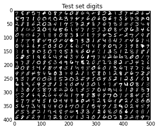
test_set_img = util.mosaic(25, digits[train_n:])
plt.title('Test set digits')
plt.imshow(test_set_img, cmap='binary_r')
<matplotlib.image.AxesImage at 0x7fd3ee2e4990>
Now, it’s time to construct classifiers. We will use a SVM classifier with an RBF kernel, i.e. \(\kappa(\mathbf{u},\mathbf{v}) = \exp(-\gamma\|\mathbf{u}-\mathbf{v}\|^2)\). Such an SVM has two hyperparameters that must be optimized, namely the misclassification penalty \(C\) and kernel parameter \(\gamma\).
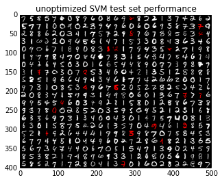
We start with an SVM with default parameters, which in this case means: \(C=1\) and \(\gamma=0.5\).
model_default = util.SVM()
model_default.train(samples_train, labels_train)
vis_default, err_default = util.evaluate_model(model_default, digits_test, samples_test, labels_test)
plt.title('unoptimized SVM test set performance')
plt.imshow(vis_default)
error: 4.20 %
confusion matrix:
[[50  0  0  0  0  0  0  0  0  0]
 [ 0 45  0  0  1  0  0  0  0  0]
 [ 0  0 43  1  0  0  0  0  3  1]
 [ 0  0  0 48  0  1  0  1  0  0]
 [ 0  0  0  0 52  0  2  0  1  1]
 [ 0  0  0  0  0 49  0  0  0  0]
 [ 0  0  0  0  0  0 48  0  0  0]
 [ 0  0  1  3  0  0  0 54  0  0]
 [ 0  1  0  0  0  2  0  0 50  0]
 [ 1  0  0  0  0  0  0  1  0 40]]
<matplotlib.image.AxesImage at 0x7fd3ee288ad0>
Next, we will construct a model with optimized hyperparameters. First we need to build Optunity’s objective function. We will use 5-fold cross-validated error rate as loss function, which we will minimize.
@optunity.cross_validated(x=samples_train, y=labels_train, num_folds=5)
def svm_error_rate(x_train, y_train, x_test, y_test, C, gamma):
    model = util.SVM(C=C, gamma=gamma)
    model.train(x_train, y_train)
    resp = model.predict(x_test)
    error_rate = (y_test != resp).mean()
    return error_rate
We will use Optunity’s default solver to optimize the error rate given \(0 < C < 5\) and \(0 < \gamma < 10\) and up to 50 function evaluations. This may take a while.
optimal_parameters, details, _ = optunity.minimize(svm_error_rate, num_evals=50,
                                                   C=[0, 5], gamma=[0, 10])
# the above line can be parallelized by adding `pmap=optunity.pmap`
# however this is incompatible with IPython

print("Optimal parameters: C=%1.3f, gamma=%1.3f" % (optimal_parameters['C'], optimal_parameters['gamma']))
print("Cross-validated error rate: %1.3f" % details.optimum)
Optimal parameters: C=1.798, gamma=6.072
Cross-validated error rate: 0.025
Finally, we train a model with the optimized parameters and determine its test set performance.
model_opt = util.SVM(**optimal_parameters)
model_opt.train(samples_train, labels_train)
vis_opt, err_opt = util.evaluate_model(model_opt, digits_test, samples_test, labels_test)
plt.title('optimized SVM test set performance')
plt.imshow(vis_opt)
error: 2.80 %
confusion matrix:
[[50  0  0  0  0  0  0  0  0  0]
 [ 0 45  0  0  1  0  0  0  0  0]
 [ 0  0 44  1  0  0  0  1  1  1]
 [ 0  0  0 49  0  0  0  1  0  0]
 [ 0  0  1  0 53  0  2  0  0  0]
 [ 0  0  0  0  0 49  0  0  0  0]
 [ 0  0  0  0  0  0 48  0  0  0]
 [ 0  0  2  0  0  0  0 56  0  0]
 [ 0  1  0  0  0  1  0  0 51  0]
 [ 0  0  0  0  0  0  0  1  0 41]]
<matplotlib.image.AxesImage at 0x7fd3ee4da050>
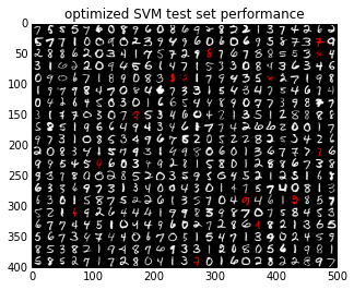
print("Reduction in error rate by optimizing hyperparameters: %1.1f%%" % (100.0 - 100.0 * err_opt / err_default))
Reduction in error rate by optimizing hyperparameters: 33.3%