Basic: minimizing a simple function

In this example we will use various Optunity solvers to minimize the following simple 2d parabola:

\[f(x, y) = (x - x_{off})^2 + (y - y_{off})^2,\]

where \(x_{off}\) and \(y_{off}\) are randomly determined offsets.

def create_objective_function():
    xoff = random.random()
    yoff = random.random()
    def f(x, y):
        return (x - xoff)**2 + (y - yoff)**2
    return f

We start with the necessary imports.

 # comment this line when running the notebook yourself
%matplotlib inline

import math
import optunity
import random
import numpy as np
import matplotlib.pyplot as plt
import matplotlib.ticker as ticker

First we check which solvers are available. This is available via optunity.available_solvers.

solvers = optunity.available_solvers()
print('Available solvers: ' + ', '.join(solvers))

Available solvers: particle swarm, tpe, sobol, nelder-mead, random search, cma-es, grid search

To run an experiment, we start by generating an objective function.

f = create_objective_function()

Now we use every available solver to optimize the objective function within the box \(x\in\ ]-5, 5[\) and \(y\in\ ]-5, 5[\) and save the results.

logs = {}
for solver in solvers:
    pars, details, _ = optunity.minimize(f, num_evals=100, x=[-5, 5], y=[-5, 5], solver_name=solver)
    logs[solver] = np.array([details.call_log['args']['x'],
                             details.call_log['args']['y']])

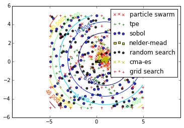
Finally, lets look at the results, that is the trace of each solver along with contours of the objective function.

# make sure different traces are somewhat visually separable
colors =  ['r', 'g', 'b', 'y', 'k', 'y', 'r', 'g']
markers = ['x', '+', 'o', 's', 'p', 'x', '+', 'o']

# compute contours of the objective function
delta = 0.025
x = np.arange(-5.0, 5.0, delta)
y = np.arange(-5.0, 5.0, delta)
X, Y = np.meshgrid(x, y)
Z = f(X, Y)

CS = plt.contour(X, Y, Z)
plt.clabel(CS, inline=1, fontsize=10, alpha=0.5)
for i, solver in enumerate(solvers):
    plt.scatter(logs[solver][0,:], logs[solver][1,:], c=colors[i], marker=markers[i], alpha=0.80)

plt.xlim([-5, 5])
plt.ylim([-5, 5])
plt.axis('equal')
plt.legend(solvers)
plt.show()

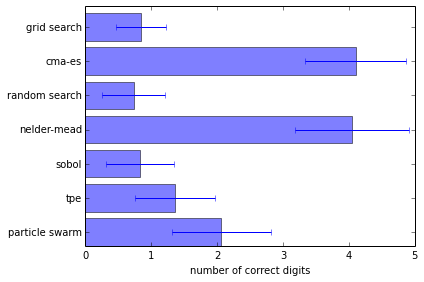
Now lets see the performance of the solvers across in 100 repeated experiments. We will do 100 experiments for each solver and then report the resulting statistics. This may take a while to run.

optima = dict([(s, []) for s in solvers])
for i in range(100):
    f = create_objective_function()

    for solver in solvers:
        pars, details, _ = optunity.minimize(f, num_evals=100, x=[-5, 5], y=[-5, 5],
                                             solver_name=solver)
        # the above line can be parallelized by adding `pmap=optunity.pmap`
        # however this is incompatible with IPython

        optima[solver].append(details.optimum)
        logs[solver] = np.array([details.call_log['args']['x'],
                                 details.call_log['args']['y']])

from collections import OrderedDict
log_optima = OrderedDict()
means = OrderedDict()
std = OrderedDict()
for k, v in optima.items():
    log_optima[k] = [-math.log10(val) for val in v]
    means[k] = sum(log_optima[k]) / len(v)
    std[k] = np.std(log_optima[k])

plt.barh(np.arange(len(means)), means.values(), height=0.8, xerr=std.values(), alpha=0.5)
plt.xlabel('number of correct digits')
plt.yticks(np.arange(len(means))+0.4, list(means.keys()))
plt.tight_layout()
plt.show()