Optimization response surface
In this example we will use Optunity to optimize hyperparameters for a support vector machine classifier (SVC) in scikit-learn. We will construct a simple toy data set to illustrate that the response surface can be highly irregular for even simple learning tasks (i.e., the response surface is non-smooth, non-convex and has many local minima).
import optunity
import optunity.metrics

# comment this line if you are running the notebook
import sklearn.svm
import numpy as np
import math
import pandas

%matplotlib inline
from matplotlib import pylab as plt
from mpl_toolkits.mplot3d import Axes3D
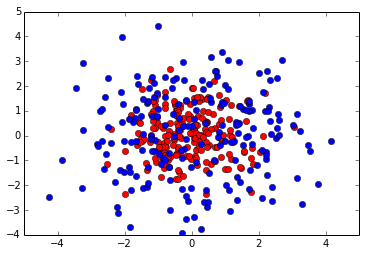
Create a 2-D toy data set.
npos = 200
nneg = 200

delta = 2 * math.pi / npos
radius = 2
circle = np.array(([(radius * math.sin(i * delta),
                     radius * math.cos(i * delta))
                    for i in range(npos)]))

neg = np.random.randn(nneg, 2)
pos = np.random.randn(npos, 2) + circle

data = np.vstack((neg, pos))
labels = np.array([False] * nneg + [True] * npos)
Lets have a look at our 2D data set.
plt.plot(neg[:,0], neg[:,1], 'ro')
plt.plot(pos[:,0], pos[:,1], 'bo')
[<matplotlib.lines.Line2D at 0x7f1f2a6a2b90>]
In order to use Optunity to optimize hyperparameters, we start by defining the objective function. We will use 5-fold cross-validated area under the ROC curve. We will regenerate folds for every iteration, which helps to minimize systematic bias originating from the fold partitioning.
We start by defining the objective function svm_rbf_tuned_auroc(),
which accepts \(C\) and \(\gamma\) as arguments.
@optunity.cross_validated(x=data, y=labels, num_folds=5, regenerate_folds=True)
def svm_rbf_tuned_auroc(x_train, y_train, x_test, y_test, logC, logGamma):
    model = sklearn.svm.SVC(C=10 ** logC, gamma=10 ** logGamma).fit(x_train, y_train)
    decision_values = model.decision_function(x_test)
    auc = optunity.metrics.roc_auc(y_test, decision_values)
    return auc
Now we can use Optunity to find the hyperparameters that maximize AUROC.
optimal_rbf_pars, info, _ = optunity.maximize(svm_rbf_tuned_auroc, num_evals=300, logC=[-4, 2], logGamma=[-5, 0])
# when running this outside of IPython we can parallelize via optunity.pmap
# optimal_rbf_pars, _, _ = optunity.maximize(svm_rbf_tuned_auroc, 150, C=[0, 10], gamma=[0, 0.1], pmap=optunity.pmap)

print("Optimal parameters: " + str(optimal_rbf_pars))
print("AUROC of tuned SVM with RBF kernel: %1.3f" % info.optimum)
Optimal parameters: {'logGamma': -1.7262599731822696, 'logC': 0.5460942232689681}
AUROC of tuned SVM with RBF kernel: 0.825
We can turn the call log into a pandas dataframe to efficiently inspect the solver trace.
df = optunity.call_log2dataframe(info.call_log)
The past function evaluations indicate that the response surface is filled with local minima, caused by finite sample effects. To see this, we can make surface plots.
cutoff = 0.5
fig = plt.figure()
ax = fig.add_subplot(111, projection='3d')
ax.scatter(xs=df[df.value > cutoff]['logC'],
           ys=df[df.value > cutoff]['logGamma'],
           zs=df[df.value > cutoff]['value'])
ax.set_xlabel('logC')
ax.set_ylabel('logGamma')
ax.set_zlabel('AUROC')
<matplotlib.text.Text at 0x7f1f26cbed50>
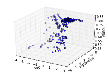
The above plot shows the particles converge directly towards the optimum. At this granularity, the response surface appears smooth.
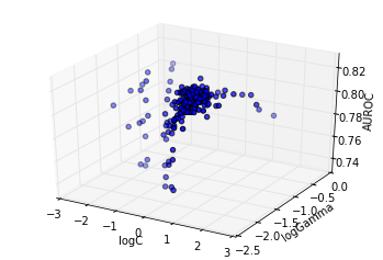
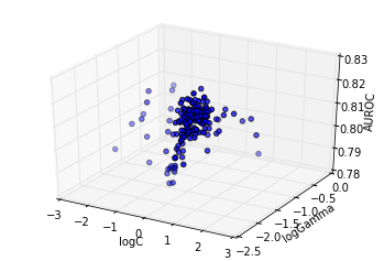
However, a more detailed analysis reveals this is not the case, as shown subsequently: - showing the sub trace with score up to 90% of the optimum - showing the sub trace with score up to 95% of the optimum - showing the sub trace with score up to 99% of the optimum
cutoff = 0.9 * info.optimum
fig = plt.figure()
ax = fig.add_subplot(111, projection='3d')
ax.scatter(xs=df[df.value > cutoff]['logC'],
           ys=df[df.value > cutoff]['logGamma'],
           zs=df[df.value > cutoff]['value'])
ax.set_xlabel('logC')
ax.set_ylabel('logGamma')
ax.set_zlabel('AUROC')
<matplotlib.text.Text at 0x7f1f2a5c3190>
cutoff = 0.95 * info.optimum
fig = plt.figure()
ax = fig.add_subplot(111, projection='3d')
ax.scatter(xs=df[df.value > cutoff]['logC'],
           ys=df[df.value > cutoff]['logGamma'],
           zs=df[df.value > cutoff]['value'])
ax.set_xlabel('logC')
ax.set_ylabel('logGamma')
ax.set_zlabel('AUROC')
<matplotlib.text.Text at 0x7f1f26ae5410>
Lets further examine the area close to the optimum, that is the 95% region. We will examine a 50x50 grid in this region.
minlogc = min(df[df.value > cutoff]['logC'])
maxlogc = max(df[df.value > cutoff]['logC'])
minloggamma = min(df[df.value > cutoff]['logGamma'])
maxloggamma = max(df[df.value > cutoff]['logGamma'])

_, info_new, _ = optunity.maximize(svm_rbf_tuned_auroc, num_evals=2500,
                                   logC=[minlogc, maxlogc],
                                   logGamma=[minloggamma, maxloggamma],
                                   solver_name='grid search')
Make a new data frame of the call log for easy manipulation.
df_new = optunity.call_log2dataframe(info_new.call_log)
Determine the region in which we will do a standard grid search to obtain contours.
reshape = lambda x: np.reshape(x, (50, 50))
logcs = reshape(df_new['logC'])
loggammas = reshape(df_new['logGamma'])
values = reshape(df_new['value'])
Now, lets look at a contour plot to see whether or not the response surface is smooth.
levels = np.arange(0.97, 1.0, 0.005) * info_new.optimum
CS = plt.contour(logcs, loggammas, values, levels=levels)
plt.clabel(CS, inline=1, fontsize=10)
plt.title('Contours of SVM tuning response surface')
plt.xlabel('log C')
plt.ylabel('log gamma')
/usr/lib/pymodules/python2.7/matplotlib/contour.py:483: DeprecationWarning: using a non-integer number instead of an integer will result in an error in the future
  nlc.append(np.r_[lc[:I[0] + 1], xy1])
/usr/lib/pymodules/python2.7/matplotlib/contour.py:485: DeprecationWarning: using a non-integer number instead of an integer will result in an error in the future
  nlc.append(np.r_[xy2, lc[I[1]:]])
/usr/lib/pymodules/python2.7/matplotlib/contour.py:479: DeprecationWarning: using a non-integer number instead of an integer will result in an error in the future
  nlc.append(np.r_[xy2, lc[I[1]:I[0] + 1], xy1])
/usr/lib/pymodules/python2.7/matplotlib/contour.py:479: DeprecationWarning: using a non-integer number instead of an integer will result in an error in the future
  nlc.append(np.r_[xy2, lc[I[1]:I[0] + 1], xy1])
/usr/lib/pymodules/python2.7/matplotlib/contour.py:479: DeprecationWarning: using a non-integer number instead of an integer will result in an error in the future
  nlc.append(np.r_[xy2, lc[I[1]:I[0] + 1], xy1])
/usr/lib/pymodules/python2.7/matplotlib/contour.py:479: DeprecationWarning: using a non-integer number instead of an integer will result in an error in the future
  nlc.append(np.r_[xy2, lc[I[1]:I[0] + 1], xy1])
/usr/lib/pymodules/python2.7/matplotlib/contour.py:483: DeprecationWarning: using a non-integer number instead of an integer will result in an error in the future
  nlc.append(np.r_[lc[:I[0] + 1], xy1])
/usr/lib/pymodules/python2.7/matplotlib/contour.py:485: DeprecationWarning: using a non-integer number instead of an integer will result in an error in the future
  nlc.append(np.r_[xy2, lc[I[1]:]])
/usr/lib/pymodules/python2.7/matplotlib/contour.py:479: DeprecationWarning: using a non-integer number instead of an integer will result in an error in the future
  nlc.append(np.r_[xy2, lc[I[1]:I[0] + 1], xy1])
/usr/lib/pymodules/python2.7/matplotlib/contour.py:479: DeprecationWarning: using a non-integer number instead of an integer will result in an error in the future
  nlc.append(np.r_[xy2, lc[I[1]:I[0] + 1], xy1])
<matplotlib.text.Text at 0x7f1f26ac3090>
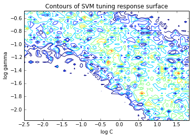
Clearly, this response surface is filled with local minima. This is a general observation in automated hyperparameter optimization, and is one of the key reasons we need robust solvers. If there were no local minima, a simple gradient-descent-like solver would do the trick.